[论文精读]Multi-View Multi-Graph Embedding for Brain Network Clustering Analysis_电脑知识

[论文精读]Multi-View Multi-Graph Embedding for Brain Network Clustering Analysis

创始人

2024-11-12 09:37:16

论文原文：3504035.3504050 (acm.org)

英文是纯手打的！论文原文的summarizing and paraphrasing。可能会出现难以避免的拼写错误和语法错误，若有发现欢迎评论指正！文章偏向于笔记，谨慎食用

1. 省流版

1.1. 心得

1.2. 论文总结图

2. 论文逐段精读

2.1. Abstract

2.2. Introduction

2.3. Related work

2.4. Preliminaries

2.5. Methodology

2.5.1. Problem definition

2.5.2. M2E approach

2.5.3. Optimization framework

2.6. Experiments and evaluation

2.6.1. Data collection and preprocessing

2.6.2. Baselines and metrics

2.6.3. Clustering results

2.6.4. Parameter sensitivity analysis

2.6.5. Factor analysis

2.7. Conclusion

3. 知识补充

3.1. 偏对称张量

4. Reference

1. 省流版

1.1. 心得

（1）这个好像不是深度学习捏~

1.2. 论文总结图

2. 论文逐段精读

2.1. Abstract

①They proposed a Multi-view Multigraph Embedding (M2E) to get information from different views

2.2. Introduction

①The conceptual view of M2E:

2.3. Related work

①Introducing graph embedding methods

②Compared with multi-view clustering and multi-view embedding

2.4. Preliminaries

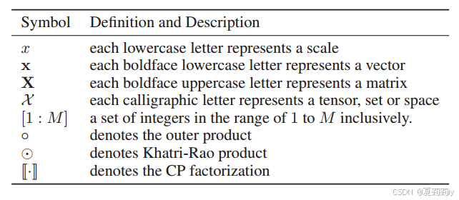
①Notations:

②Definition 1: introducing partial symmetric tensor（不过我觉得作者没有解释地很清楚，他说“如果一个M阶张量在模态1到M上偏对称，那么它就是秩一偏对称张量”。不如看看我的知识补充）

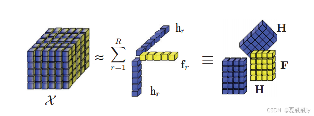
③Definition 2: matricize tensor $\mathcal{X}\in\mathbb{R}^{I_{1}\times\cdots\times I_{M}}$ to $\mathbf{X}_{(m)}\in \mathbb{R}^{I_m\times J}$ , where

$\begin{aligned}&j=1+\sum_{p=1,p\neq m}^{M}(i_{p}-1)J_{p}, with\\&J_{p}=\begin{cases}1,&if p=1 or (p=2 and m=1)\\\Pi_{q=1,q\neq m}^{p-1}I_q,&otherwise.\end{cases}\end{aligned}$

④Definition 3: factorize $\mathcal{X}\in\mathbb{R}^{I_{1}\times\cdots\times I_{M}}$ to:

$\mathcal{X}\approx\sum_{r=1}^R\mathbf{x}_r^{(1)}\circ\cdots\circ\mathbf{x}_r^{(M)}\equiv[[\mathbf{X}^{(1)},...,\mathbf{X}^{(M)}]]$

which needs to minimize the estimation error:

$\mathcal{L}=\min_{\mathbf{X}^{(1)},\cdots,\mathbf{X}^{(M)}}\lVert\mathcal{X}-[[\mathbf{X}^{(1)},\cdots,\mathbf{X}^{(M)}]]\rVert_F^2$

and, to solve non convex optimization problems:

$\mathbf{X}^{(k)}\leftarrow\arg\min_{\mathbf{X}^{(k)}}\|\mathbf{X}_{(k)}-\mathbf{X}^{(k)}(\odot_{i\neq k}^n\mathbf{X}^{(i)})^\mathrm{T}\|_F^2$

where $\odot_{i\neq k}^{M}\mathbf{X}^{(i)}=\mathbf{X}^{(M)}\odot\cdots\mathbf{X}^{(k-1)}\odot\mathbf{X}^{(k+1)}\cdots\odot\mathbf{X}^{(1)}$

2.5. Methodology

2.5.1. Problem definition

①For samples with views, they have brain connectivity $\mathbf{W}\in\mathbb{R}^{M\times M}$ each with nodes

②For each view, the whole graph set is $\mathcal{D}^{(v)}=\{\mathbf{W}_{1}^{(v)},\mathbf{W}_{2}^{(v)},\cdots,\mathbf{W}_{N}^{(v)}\}$

③All the views: $\mathcal{D} = \{\mathcal{D}^{(1)},\mathcal{D}^{(2)},\cdots,\mathcal{D}^{(V)}\}$

④To learn an embedding $\mathbf{F}^*\in\mathbb{R}^{N\times R}$ for each participant

2.5.2. M2E approach

①Concatenated third-order tensor:

$\mathcal{X}^{(v)}=[\mathbf{W}_1^{(v)},\mathbf{W}_2^{(v)},\cdots,\mathbf{W}_N^{(v)}]\in \mathbb{R}^{M\times M\times N},v \in [1 : V]$

②Embedding function:

$\min_{\mathbf{H}^{(v)},\mathbf{F}^{(v)}}\sum_{v=1}^V||\mathcal{X}^{(v)}-[[\mathbf{H}^{(v)},\mathbf{H}^{(v)},\mathbf{F}^{(v)}]]||_F^2$

where $\mathbf{H}^{(v)}\in\mathbb{R}^{M\times R}$ and $\mathbf{F}^{(v)}\in\mathbb{R}^{N\times R}$ calculated by CP factorization:

③Common embedding learning:

$\min_{\mathbf{F}^*}\sum_{v=1}^V\lambda_v||\mathbf{F}^{(v)}-\mathbf{F}^*||_F^2$

④Combining them to optimize M2E:

$\begin{aligned}\mathcal{O}&=\min_{\mathbf{H}^{(v)},\mathbf{F}^{*},\mathbf{F}^{(v)}}\sum_{v=1}^{V}||\mathcal{X}^{(v)}-[[\mathbf{H}^{(v)},\mathbf{H}^{(v)},\mathbf{F}^{(v)}]]||_{F}^{2}\\&+\sum_{v=1}^{V}\lambda_{v}||\mathbf{F}^{(v)}-\mathbf{F}^{*}||_{F}^{2}\end{aligned}$

where the first term is for minimize the dependence of multi-graphs and the second is for multi-views

2.5.3. Optimization framework

①Parameter needs estimate: $\mathbf{H}^{(v)}\in\mathbb{R}^{M\times R}$ , $\mathbf{F }^{(v)}\in\mathbb{R}^{N\times R}$ , and $\mathbf{F}^{*}\in\mathbb{R}^{N\times R}$ . Due to they are not convex, no closed-form adopted. Then they introduced an iteration method, Alternating Direction Method of Multipliers (ADMM) approach.

②They use variable substitution technique, fixing $\mathbf{F }^{(v)}$ and $\mathbf{F}^{*}$ , compute $\mathbf{H}^{(v)}$ :

$\begin{aligned}&\min_{\mathbf{H}^{(v)},\mathbf{P}^{(v)}}||\mathcal{X}^{(v)}-[[\mathbf{H}^{(v)},\mathbf{P}^{(v)},\mathbf{F}^{(v)}]]||_{F}^{2}\\&s.t. \mathbf{H}^{(v)}= \mathbf{P}^{(v)}\end{aligned}$

the Lagragian function:

$\mathcal{L}(\mathbf{H}^{(v)},\mathbf{P}^{(v)})=\|\mathcal{X}^{(v)}-[\mathbf{H}^{(v)},\mathbf{P}^{(v)},\mathbf{F}^{(v)}]\|_{F}^{2}\\+tr(\mathbf{U}^{(v)T}(\mathbf{H}^{(v)}-\mathbf{P}^{(v)}))+\frac{\mu}{2}\|\mathbf{H}^{(v)}-\mathbf{P}^{(v)}\|_{F}^{2}$

where $\mathbf{U}^{(v)}\in\mathbb{R}^{M\times R}$ denotes Lagrange multipliers, $\mu$ denotes penalty parameter. Optimization problem:

$\min_{\mathbf{H}^{(v)}}||\mathbf{X}_{(1)}^{(v)}-\mathbf{H}^{(v)}\mathbf{D}^{(v)\text{T}}||_F^2+\frac{\mu}{2}||\mathbf{H}^{(v)}-\mathbf{P}^{(v)}+\frac{1}{\mu}\mathbf{U}^{(v)}||_F^2$

they transfer $\mathcal{X}^{(v)}$ to $\mathbf{X}_{(1)}^{(v)}\in\mathbb{R}^{M\times(MN)}$ , and define $\mathbf{D}^{(v)}=\mathbf{F}^{(v)}\odot\mathbf{P}^{(v)}\in\mathbb{R}^{(NM)\times R}$

. Further changing the minimizing function:

$\min_{\mathbf{H}^{(v)}}tr(\mathbf{H}^{(v)}\mathbf{A}^{(v)}\mathbf{H}^{(v)^{\mathrm{T}}})-tr(\mathbf{B}^{(v)^{\mathrm{T}}}\mathbf{H}^{(v)})$

where $\mathbf{A}^{(v)}=\mathbf{D}^{(v)^{\mathrm{T}}}\mathbf{D}^{(v)}+\frac{\mu}{2}\mathbf{I}$ and $\mathbf{B}^{(v)}=2\mathbf{X}_{(1)}^{(v)}\mathbf{D}^{(v)}+\mu\mathbf{P}^{(v)}-\mathbf{U}^{(v)}$ . Solving it by update $\mathbf{H}^{(v)}$ :

$\mathbf{H}_{t+1}^{(v)}\leftarrow\mathbf{H}_t^{(v)}-\frac1{L^{(v)}}(2\mathbf{H}^{(v)^\mathrm{T}}\mathbf{A}^{(v)}-\mathbf{B}^{(v)})$

where $L^{(v)}$ denotes Lipschitz coefficient and equals to the maximum eigenvalue of $2\mathbf{A}^{(v)}$ . They applied Khatri-Rao product to calculate $\mathbf{D}^{(v)^\mathrm{T}}\mathbf{D}^{(v)}$ :

$\begin{aligned} \mathbf{D}^{(v)^{\mathrm{T}}}\mathbf{D}^{(v)}& =(\mathbf{F}^{(v)}\odot\mathbf{P}^{(v)^{\mathrm{T}}})(\mathbf{F}^{(v)}\odot\mathbf{P}^{(v)}) \\ &=(\mathbf{F}^{(v)^{\mathrm{T}}}\mathbf{F}^{(v)})*(\mathbf{P}^{(v)^{\mathrm{T}}}\mathbf{P}^{(v)}) \end{aligned}$

where $\ast$ denotes Hadamard product. The updating function of $\mathrm{P}^{(v)}$ :

$\mathbf{P}_{t+1}^{(v)}\leftarrow\mathbf{P}_t^{(v)}-\frac1{L^{(v)}}(2\mathbf{P}_t^{(v)}\mathbf{A}^{(v)}-\mathbf{B}^{(v)})$

where $\mathbf{A}^{(v)}=\mathbf{E}^{(v)^{\mathrm{T}}}\mathbf{E}^{(v)}+\frac\mu2(\mathbf{I})$ , $\mathbf{B}^{(v)}=2\mathbf{X}_{(2)}^{(v)}\mathbf{E}^{(v)}+\mu\mathbf{H}^{(v)}+\mathbf{U}^{(v)}$ , $\mathbf{E}^{(v)}=\mathbf{F}^{(v)}\odot\mathbf{H}^{(v)}\in\mathbb{R}^{(NM)\times R}$ . Lastly update $\mathrm{U}(v)$ :

$\mathbf{U}_t^{(v)}\leftarrow\mathbf{U}_t^{(v)}+\mu(\mathbf{H}^{(v)}-\mathbf{P}^{(v)})$

③Then they fix $\mathbf{F}^{*}$ and $\mathbf{H}^{(v)}$ to compute $\mathbf{F }^{(v)}$ by minimize:

$\min_{\mathbf{F}^{(v)}} ||\mathbf{X}_{(3)}^{(v)}-\mathbf{F}^{(v)}\mathbf{J}^{(v)^{\mathrm{T}}}||_{F}^{2}+\lambda_{(v)}||\mathbf{F}^{(v)}-\mathbf{F}^{*}||_{F}^{2}$

where $\mathbf{J}^{(v)}=\mathbf{P}^{(v)}\odot\mathbf{H}^{(v)}\in\mathbb{R}^{(MM)\times R}$ . The updating function of $\mathbf{F }^{(v)}$ :

$\mathbf{F}_{t+1}^{(v)}\leftarrow\mathbf{F}_t^{(v)}-\frac{1}{L^{(v)}}(2\mathbf{F}_t^{(v)}\mathbf{A}^{(v)}-\mathbf{B}^{(v)})$

where $\mathbf{A}^{(v)} = \mathbf{J}^{(v)^\mathrm{T}}\mathbf{J}^{(v)} + \lambda_{(v)}(\mathbf{I})$ , $\mathbf{B}^{v} = 2\mathbf{X}_{(3)}^{(v)}\mathbf{J}^{(v)} +2\lambda_{(v)}\mathbf{F}^*$

④Finally, they fix $\mathbf{H}^{(v)}$ and $\mathbf{F }^{(v)}$ to minimize ${\mathcal{O}}$ over $\mathbf{F}^{*}$ :

$\mathbf{F}^*=\frac{\sum_{v=1}^V\lambda_{(v)}\mathbf{F}^{(v)}}{\sum_{v=1}^V\lambda_{(v)}}$

⑤Overall time complexity:

$O(MaxIter(R^{3}+R^{2}(2M+N+1)+(M^{2}N+M+NV)R)V)$

2.6. Experiments and evaluation

2.6.1. Data collection and preprocessing

（1）Human Immunodeficiency Virus Infection (HIV)

①Sample: randomly select 35 patients and 35 controls from dataset due to the data imbalance

②Atlas: AAL 90

（2）Bipolar Disorder (BP)

①Sample: 52 BP and 45 controls

②Atlas: self-generated 82 regions

euthymia n. 情感正常

2.6.2. Baselines and metrics

①Introducing compared models

②Grid search for hyper-parameters: $\lambda _1,\lambda _2\in\{10^{-4},10^{-2},...,10^{4}\}$ , form $\{1,2,...,20\}$

2.6.3. Clustering results

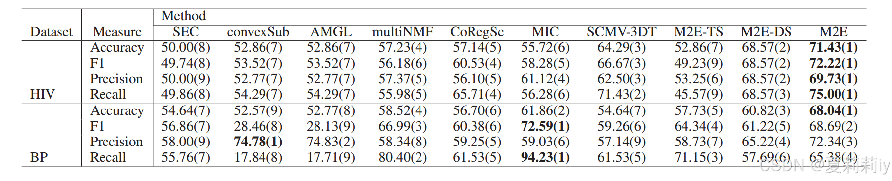
①Performance comparison table:

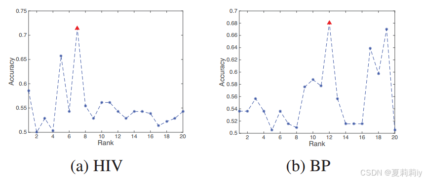
2.6.4. Parameter sensitivity analysis

①Ablation on $\lambda$ :

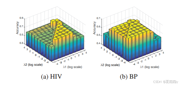
②Ablation on :

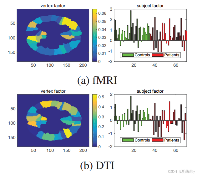
2.6.5. Factor analysis

①The activity intensity of the brain region and the embedded feature $\mathbf{F }^{(v)}$ :

2.7. Conclusion

They design a novel multi-view multi-graph embedding framework based on partially-symmetric tensor factorization

3. 知识补充

3.1. 偏对称张量

（1）定义：偏对称张量是指张量中的某些分量在特定的下标重排后，其值保持不变。这种性质与张量的对称性有关，但与完全对称的张量（即所有下标重排后元素都相等的张量）不同，偏对称张量只要求部分下标重排后元素相等。

（2）示例：以三阶张量为例，如果满足以下条件之一或多个，则可以称为偏对称张量：

① $x_{ijk}=x_{jik}$ （第一个和第二个下标互换）

② $x_{ijk}=x_{kji}$ （第一个和第三个下标互换）

③ $x_{ijk}=x_{jik}=x_{kij}$ （同时满足前两个条件）

4. Reference

Liu, Y. et al. (2018) 'Multi-View Multi-Graph Embedding for Brain Network Clustering Analysis', AAAI. doi: https://doi.org/10.48550/arXiv.1806.07703

上一篇：recovernt3.5破解版-警惕！RecoverNT3.5 破解版背后的猫腻，你知道多少？

下一篇：全国新生儿重名查询：名字千奇百怪仍有重名，家长取名费尽心思也难避免

[论文精读]Multi-View Multi-Graph Embedding for Brain Network Clustering Analysis

1. 省流版

1.1. 心得

1.2. 论文总结图

2. 论文逐段精读

2.1. Abstract

2.2. Introduction

2.3. Related work

2.4. Preliminaries

2.5. Methodology

2.5.1. Problem definition

2.5.2. M2E approach

2.5.3. Optimization framework

2.6. Experiments and evaluation

2.6.1. Data collection and preprocessing

2.6.2. Baselines and metrics

2.6.3. Clustering results

2.6.4. Parameter sensitivity analysis

2.6.5. Factor analysis

2.7. Conclusion

3. 知识补充

3.1. 偏对称张量

4. Reference

相关内容

热门资讯